hist(rbinom(100000,100,0.05),col="yellow") # Binomial distribution with 100 trials and a probability of success of 0.05

hist(rpois(100000,lambda=100*0.05),add=T,col="#0000ff66") # Poisson distribution with a mean of 100*0.05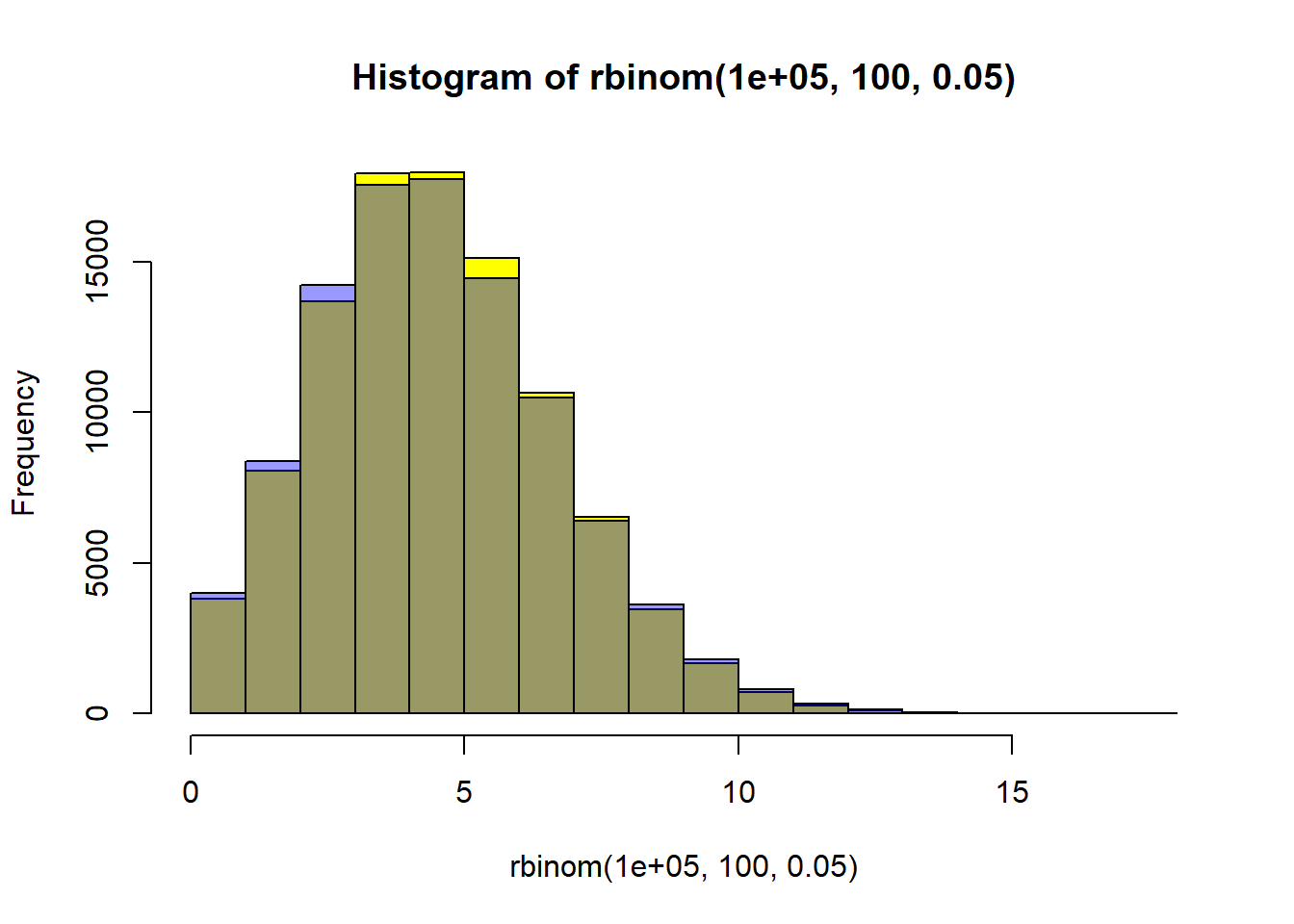
“To make sense of an observation, everybody needs a model … whether he knows it or not.”
— Marc Kéry
Linear models are typically used to try to find the relationship between a response variable and explanatory variable(s). In a ‘classic’ linear model (i.e., linear regression), the response variable is assumed to follow a Normal distribution, whose mean equals to a linear combination of the explanatory variables. Simply put, the response variable is equal to a linear combination of the covariates plus some random noise, and this random noise has a Normal distribution.
A generalization of this approach can be used when dealing with a response variable that is discrete and/or bounded. Three typical situations where this might occur:
1/ Binary: Trying to determine the probability of an event to happen. For example, one might want to model occupancy of a species of interest in a particular area (i.e. is it present or not). Our response variable would therefore be either a 0 or a 1. However, a linear regression could easily return values that are not contained in this set.
2/ Discrete and bounded: Trying to model the observation of an repeated binary event. For example, you might want to figure out what is the probability to detect an animal given that it is present in an area. To do so, you could conduct five 10-minute sessions where you will note during how many session the animal has been detected. Obviously, the amount of possible detection (binary event: detection or no detection) will be bounded between 0 and the total number of session (repeated measures). Moreover, there is no “half-detection”. I don’t care that you’re unsure if the howling you heard during session 3 was the wolf you are studying or a student caught in a bear trap, you can’t count it as a half-detection “just in case”. A regular linear model would not respect the bounding nor the fact that we have discrete values.
3/ Discrete: Trying to model a population abundance. We are counting individuals. Chances are that we are not going to find 0.24 or 17.2 or 82.7458 individuals. We are modeling a discrete number of individuals. The linear approach could not only give us half individuals in the regression, but could also lead us to predict negative numbers of individuals for certain values of the covariates.
We need a solution to accommodate those situations! Enter the GLMs! The Generalized Linear Models. (Normally, as you read that, The Ride of the Valkyries should be playing in your head.)
We are going to start with 3 typical go-to distributions (but don’t worry, we’ll later also talk about others).
The linear models we are used to aim at estimating the mean of a normal distribution for the response variable by expressing it as a result of our covariates. The normal distribution has 2 parameters: the mean, and the standard deviation. We are simply expressing the mean of the normal distribution as a linear combination of our covariates to link our explanatory variables to our response variable!
The binomial distribution will be used when facing a) a binary variable (presence/absence, success/failure, yes/no) or b) the repetition of a binary variable (number of occupied sites in a given area for example). In situation a), only one parameter is necessary to model the response variable: the event probability. In case b), two parameters are necessary: the probability of a single event, and the number of repetition. As the number of repetition is simply equal to the total of “success” and “failure”, this information is contained in the data. This leaves us with one parameter to once again model our response variable, the probability. Cool, we now just need to find a way to express this probability as a linear combination of our covariates to link our explanatory variables to our response variable!
The Poisson distribution will typically be used for population counts. It has only one parameter (‘lambda’), and make the assumption that the mean and the variance are equal. Once again, cool, we now just need to find a way to express this mean as a linear combination of our covariates to link our explanatory variables to our response variable! The Poisson distribution is basically what would happen to a binomial distribution for a really low probability (rare events) but over a really large number of trials. As a matter of fact, if we take ‘n’ trials and a probability ‘p’ of the targeted event to happen, the Poisson distribution with a mean ‘np’ can be seen as a good approximation of the binomial distribution if ‘n’ is at least 20 and ‘p’ is smaller than or equal to 0.05, and as an excellent approximation if ‘n’ is greater than or equal to 100 and the product ‘n’ by ‘p’ is lower than or equal to 10. Need proof? Here:
hist(rbinom(100000,100,0.05),col="yellow") # Binomial distribution with 100 trials and a probability of success of 0.05
hist(rpois(100000,lambda=100*0.05),add=T,col="#0000ff66") # Poisson distribution with a mean of 100*0.05In yellow, the binomial distribution. In blue, the approximating Poisson distribution. In grey(ish) the overlap between the two. Not bad, right?
We now have different distributions available to provide a statistical framework for different types of response variables. We also have a parameter for each distribution that controls it. We just need to find a function to link a linear combination of our explanatory variables to this parameter in order to model the relationship between the response variable and those covariates. This is what is called the link function.
The link function for the normal distribution is the identity function. Basically, it’s just the linear combination by itself, as we have always done so far.
The link function for the binomial distribution is the logit function. It allows to define a linear combination that varies between -\(\infty\) and +\(\infty\) and to transfer it on a 0 to 1 probability scale. For information, the logit of a probability ‘p’ is equal to the logarithm of the odds: \(\log(\frac{p}{(1-p)})\).
The link function for the poisson distribution is the log function. It makes it possible to go from a space ranging from -\(\infty\) and +\(\infty\) to a scale ranging from 0 to to +\(\infty\).
No need to worry too much about that right now, when we will specify the type of model we want to use to R, R will bundle of that together. You just need to indicate the family, and both the distribution and the corresponding link function will be selected.
Now that we can link our response variable to the explanatory variables, we just need to define the linear predictor in the same way we are used to for linear regressions. And voila! We’ll be doing GLMs in no time. Let’s practice!