5 The Negative Binomial regression

So far, so good. When we were dealing with our count data, everything matched the model’s underlying assumptions (e.g., no overdispersion, no excess of zero counts). But this is not always the case (some cynical people would use “rarely” here, but I am not like that). The next 2 chapters are going to be dedicated to how to handle those “less-than-perfect” scenarios.

First, let’s take a look at what we can do when we are faced with the dreadful presence of overdispersion. We’ve all been there, life throws a curve ball or two, things get crazy, and before we know it, we overdisperse. No need to be negative though, we have a distribution that can handle that really well: the Negative Binomial distribution. The negative binomial distribution is closely related to the Poisson distribution, but allows for the variance of the distribution (i.e., how much it “disperses”) to be larger than its mean, therefore relaxing our previously limiting assumption. It does so by incorporating an extra parameter \(\theta\) to handle the dispersion.

A typical example of a situation where a negative binomial distribution applies in ecological data relates to social animals. Let’s consider a FWC researcher studying colonial bird populations: while some areas along the coast of Florida might have few birds, others could have large clusters representing hotspots for your population of interest, leading to a higher variance than otherwise expected.

Unfortunately for us, base R does not include a function to directly handle negative binomial regressions by default (yet?). Fortunately, as always, the amazing R community stepped up and provided us with the tools needed to tackle that task. The most well-known package used to perform this job is arguably the MASS package.

library(MASS)

5.1 Data

This time, we are going to simulate some data and see if we can correctly identify what’s happening in our dataset.

Let’s look at the populations of two-toed alligators in Alabama and Florida.

# Generating state independent variable randomly
state01 <- rbinom(500, 1, 0.5)
state <- ifelse(state01==1,"Florida","Alabama")

# Setting up parameters
a <- -0.8
b <- 2.5
mu.log <- a*state01+b
mu <- exp(mu.log)

theta <-2    # Overdispersion parameter

# Generating two-toed alligator data
y=rnegbin(mu, theta = theta)  # 'rnegbin()' is coming from MASS, but this could also be done using base R with 'rnbinom()'

data.nb <- data.frame(state,y.tom=y)

# Visualizing the data
hist(data.nb$y.tom,
     breaks = 20,
     main="Two-toed alligators density plot", xlab="Recorded abundances")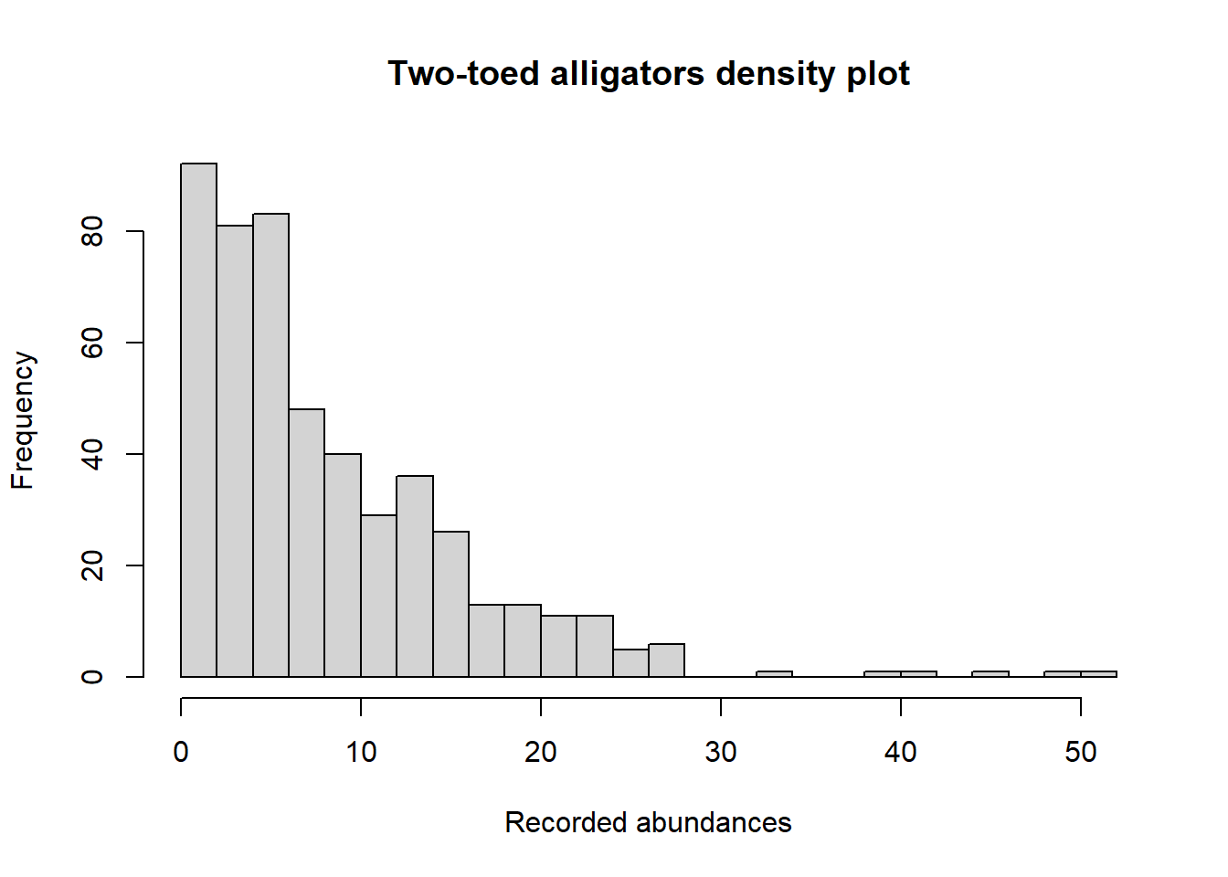

Two-toed alligators recorded abundances by State

We can even look at the details by state:

library(ggplot2)

ggplot(data.nb, aes(x=y.tom, fill=state)) +
    geom_histogram( color="#e9ecef", alpha=0.4, position = 'identity') +
    scale_fill_manual(values=c("#69b3a2", "#404080")) +
    theme_light() +
    labs(fill="") +
    xlab("Two-toed alligators abundance")+
    ylab("Count")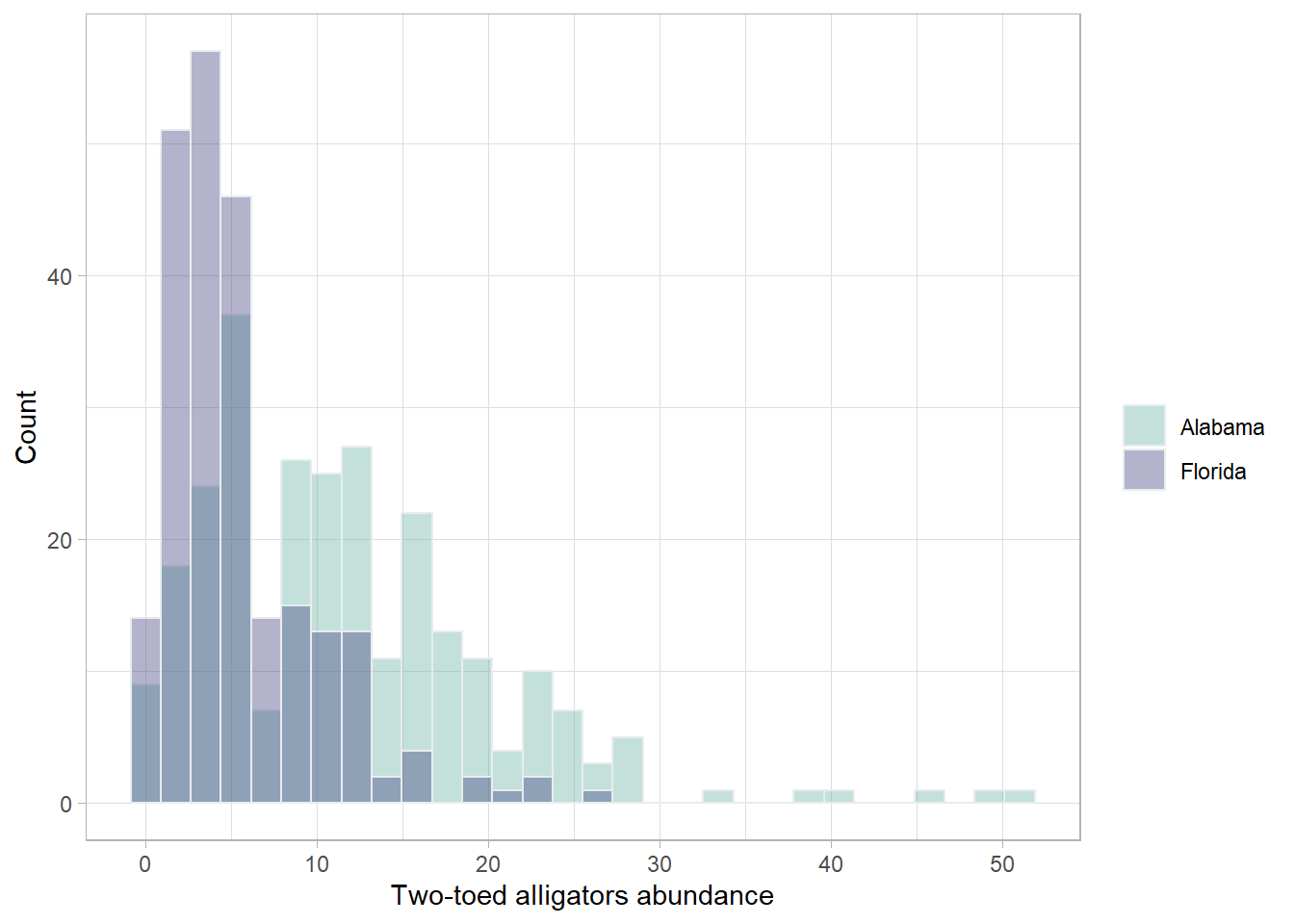

5.2 Estimation

First, let’s see if we could simply use a Poisson regression with this dataset. No need to use a bazooka if a spoon were to do the trick. We start by fitting a Poisson model, and then check for overdispersion.

Fitting the model:

tom.res.poisson=glm(y.tom~state,data=data.nb, family="poisson")
summary(tom.res.poisson)


Call:
glm(formula = y.tom ~ state, family = "poisson", data = data.nb)

Coefficients:
             Estimate Std. Error z value Pr(>|z|)    
(Intercept)   2.44938    0.01805  135.69   <2e-16 ***
stateFlorida -0.76772    0.03343  -22.96   <2e-16 ***
---
Signif. codes:  0 '***' 0.001 '**' 0.01 '*' 0.05 '.' 0.1 ' ' 1

(Dispersion parameter for poisson family taken to be 1)

    Null deviance: 2975.5  on 499  degrees of freedom
Residual deviance: 2400.5  on 498  degrees of freedom
AIC: 4187.5

Number of Fisher Scoring iterations: 5

The dispersion ratio ( \(\frac{Residual\ deviance}{Degrees\ of\ freedom}=\frac{2400.47}{498}=4.82\) ) is not encouraging… And if we more formally test for it…

library(performance)
check_overdispersion(tom.res.poisson)

# Overdispersion test

       dispersion ratio =    5.105
  Pearson's Chi-Squared = 2542.464
                p-value =  < 0.001

Overdispersion detected.

Yep, there is a clear overdispersion (which, again, is not surprising since we created those data that way… but still, it is nice to confirm it!)

So now, we got to try our chance with a negative binomial regression using the glm.nb() function from the MASS package:

tom.res.nb=glm.nb(y.tom~state,data=data.nb)
summary(tom.res.nb)


Call:
glm.nb(formula = y.tom ~ state, data = data.nb, init.theta = 2.090116582, 
    link = log)

Coefficients:
             Estimate Std. Error z value Pr(>|z|)    
(Intercept)   2.44938    0.04617   53.06   <2e-16 ***
stateFlorida -0.76772    0.07042  -10.90   <2e-16 ***
---
Signif. codes:  0 '***' 0.001 '**' 0.01 '*' 0.05 '.' 0.1 ' ' 1

(Dispersion parameter for Negative Binomial(2.0901) family taken to be 1)

    Null deviance: 671.73  on 499  degrees of freedom
Residual deviance: 554.75  on 498  degrees of freedom
AIC: 3077.2

Number of Fisher Scoring iterations: 1

              Theta:  2.090 
          Std. Err.:  0.171 

 2 x log-likelihood:  -3071.204

5.3 Diagnostics

5.3.1 Goodness of Fit: Likelihood Ratio Test

Using the likelihood ratio test (which you should feel familiar with by now), we see that our negative binomial (let’s call it NB for short, I think we’ve reach that point in our relationship with this kind of models that we are allowed to use cutesy nicknames) performs clearly better than the null model:

anova(tom.res.nb)

Analysis of Deviance Table

Model: Negative Binomial(2.0901), link: log

Response: y.tom

Terms added sequentially (first to last)

      Df Deviance Resid. Df Resid. Dev  Pr(>Chi)    
NULL                    499     671.73              
state  1   116.98       498     554.75 < 2.2e-16 ***
---
Signif. codes:  0 '***' 0.001 '**' 0.01 '*' 0.05 '.' 0.1 ' ' 1

Not only that, but because the Poisson model is technically nested within the NB model (the overdispersion parameter \(\theta\) is fixed to 1 in the case of the Poisson regression), we can also use a likelihood ratio test to see that our NB model indeed performs better than our Poisson model:

library(lmtest)

lrtest(tom.res.poisson, tom.res.nb)

Likelihood ratio test

Model 1: y.tom ~ state
Model 2: y.tom ~ state
  #Df  LogLik Df  Chisq Pr(>Chisq)    
1   2 -2091.8                         
2   3 -1535.6  1 1112.3  < 2.2e-16 ***
---
Signif. codes:  0 '***' 0.001 '**' 0.01 '*' 0.05 '.' 0.1 ' ' 1

Higher log-likelihood, significant p-value. Let’s pat ourselves on the back, we did a good job.

5.3.2 A look a the residuals

Say it with me now, our next step is to… “Make sure our residuals are distributed as expected by simulating randomized quantile residuals”. Oof, I could feel the excitement vibrating through our audience. This is tantalizing…

library(performance)
library(qqplotr)

simulated_residuals <- simulate_residuals(tom.res.nb)

plot(simulated_residuals)

Figure 5.1: Distribution of quantile residuals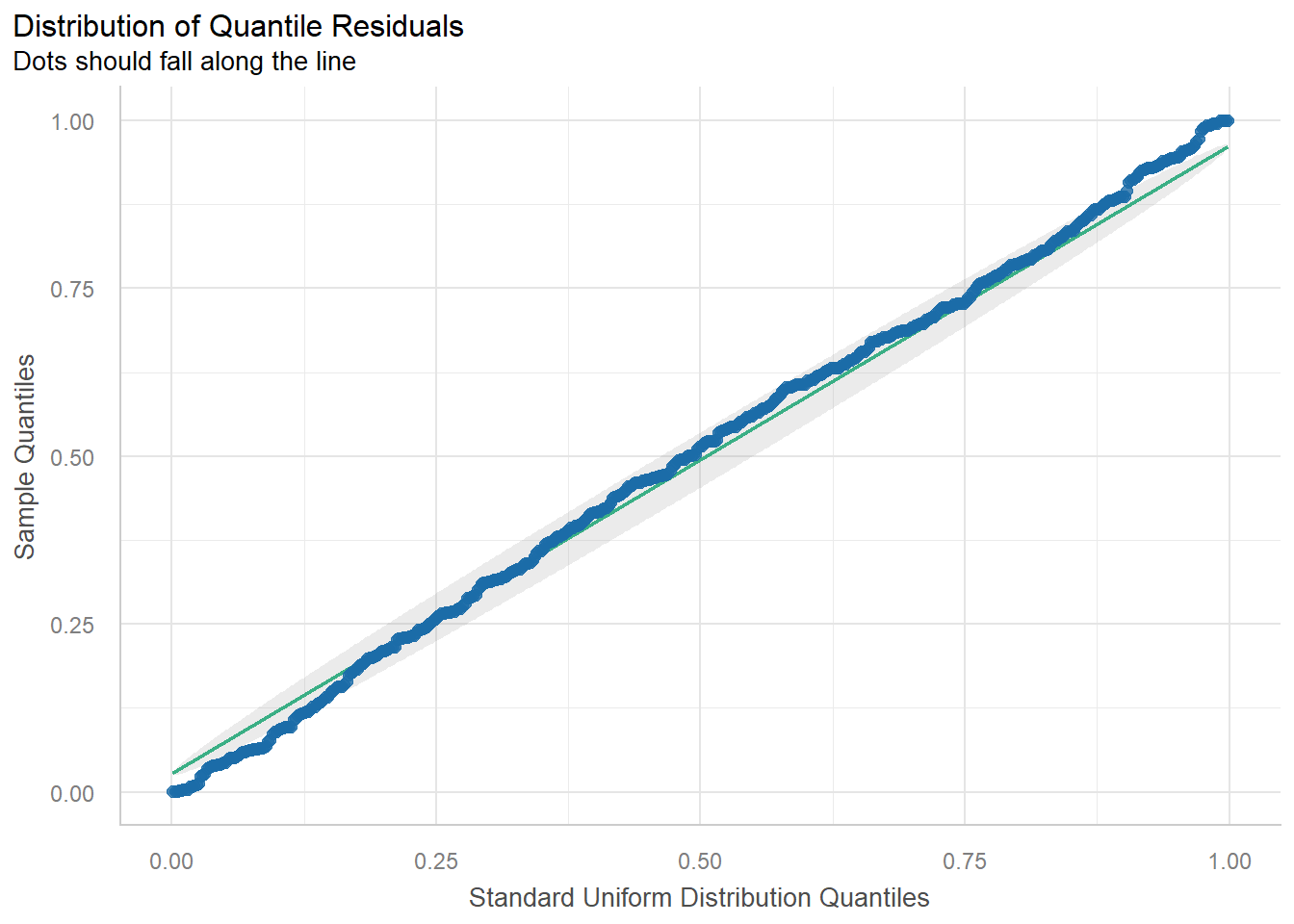

check_residuals(simulated_residuals)

OK: Simulated residuals appear as uniformly distributed (p = 0.923).

We are clear to go and make some inferences on the output of the model! Rejoice!

5.4 Inferences

summary(tom.res.nb)


Call:
glm.nb(formula = y.tom ~ state, data = data.nb, init.theta = 2.090116582, 
    link = log)

Coefficients:
             Estimate Std. Error z value Pr(>|z|)    
(Intercept)   2.44938    0.04617   53.06   <2e-16 ***
stateFlorida -0.76772    0.07042  -10.90   <2e-16 ***
---
Signif. codes:  0 '***' 0.001 '**' 0.01 '*' 0.05 '.' 0.1 ' ' 1

(Dispersion parameter for Negative Binomial(2.0901) family taken to be 1)

    Null deviance: 671.73  on 499  degrees of freedom
Residual deviance: 554.75  on 498  degrees of freedom
AIC: 3077.2

Number of Fisher Scoring iterations: 1

              Theta:  2.090 
          Std. Err.:  0.171 

 2 x log-likelihood:  -3071.204

Because the link function is typically the same as for a Poisson regression (log), interpreting coefficient of a NB regression is the same as for the Poisson regression: we just have to exponentiate the coefficient of interest.

beta.FL = coef(tom.res.nb)[["stateFlorida"]]
ci.FL = confint(tom.res.nb,"stateFlorida")
exp(c(beta.FL=beta.FL,ci.FL))

  beta.FL     2.5 %    97.5 % 
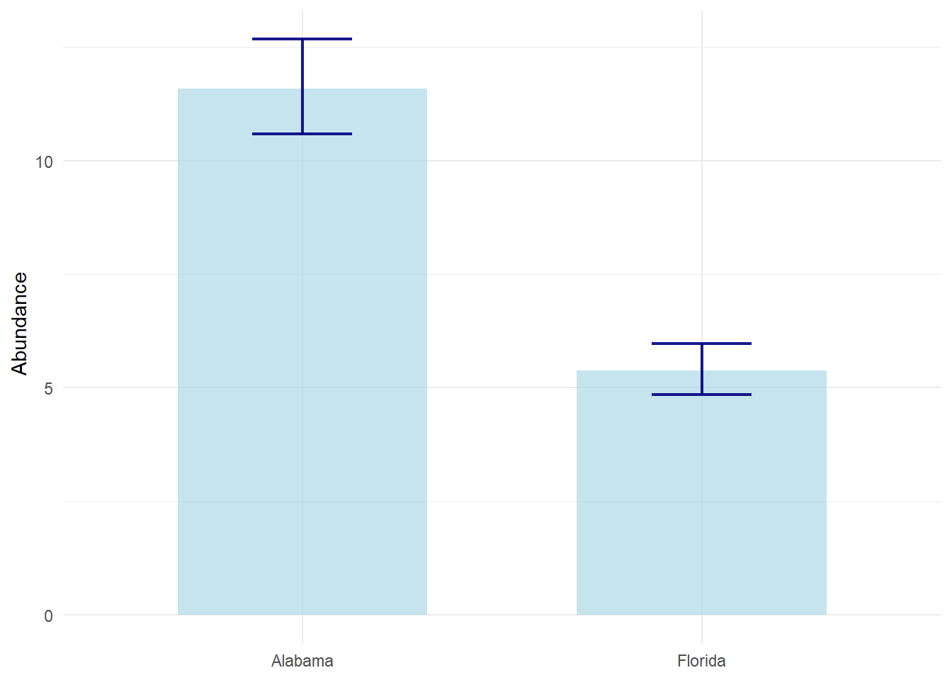
0.4640710 0.4042516 0.5327926

Our two-toed alligator population in Florida is 0.46 [0.4 ; 0.53] times that of Alabama’s, or 53.59% [46.72% ; 59.57%] smaller (i.e., \(100*(0.46-1)=-54\%\)).

5.4.1 Plotting the fit

And using the same approach as in previous chapters, we can wrap all of this up with a beautiful prediction graph (going for a more appropriate bar plot this time for good measure)!

  #| fig-cap: "Predicted mean tow-toed alligator abundance"
  
  resp.pred=data.frame(state=c("Alabama","Florida"))
  
  resp.pred$pred <- predict(tom.res.nb, newdata=resp.pred, type="response") # Predictions
  
  pred.linkscale <- predict(tom.res.nb, newdata=resp.pred, se=T) 
  pred.linkscale.CI2.5  = pred.linkscale$fit-1.96*pred.linkscale$se.fit
  pred.linkscale.CI97.5 = pred.linkscale$fit+1.96*pred.linkscale$se.fit
  
  resp.pred$CI2.5  = family(tom.res.nb)$linkinv(pred.linkscale.CI2.5)
  resp.pred$CI97.5 = family(tom.res.nb)$linkinv(pred.linkscale.CI97.5)
  
  
  library(ggplot2)
  
  ggplot(resp.pred) +
      geom_bar( aes(x=state, y=pred), stat="identity", width=5/8, fill="lightblue", alpha=0.7) +
      geom_errorbar( aes(x=state, ymin=CI2.5, ymax=CI97.5), width=1/4, color="navyblue", alpha=0.9, linewidth=0.75) +
    ylab(" Abundance") +
    theme_minimal() +
    theme(axis.title.x = element_blank())