# proportion of time we detected the species for each slope
dahu.prop <- dahu.data |> # Fun fact: |> is the base R pipe operator !
dplyr::group_by(slope) |>
dplyr::summarise(prop = mean(detect))
plot(prop~slope, data=dahu.prop) 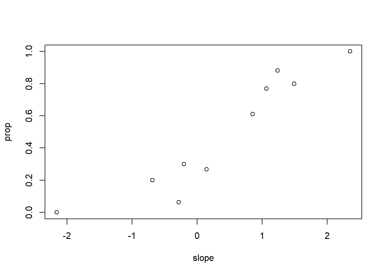
The logistic regression is the GLM used when the response variable is the result of a binomial distribution and the link function is the logit function. It is commonly used to model processes emerging from the recording of binary events (detection/non-detection, success/failure, yes/no).
Let’s take for example the repartition of the Spotted Dahu in Northern Brittany, France. We studied the presence of the dahu on 10 hills. We went on each hill a different amount of times, and each time we recorded if we were able to detect this elusive animal. We hypothesize that the presence of the dahu is related to the average slope of the hill. Here are the data (heads-up, big impractical dataset coming through):
dahu.data <-read.table(header = TRUE,
text="
site    detect           slope
   1         1       0.1458983
   1         1       0.1458983
   1         1       0.1458983
   1         1       0.1458983
   1         0       0.1458983
   1         0       0.1458983
   1         0       0.1458983
   1         0       0.1458983
   1         0       0.1458983
   1         0       0.1458983
   1         0       0.1458983
   1         0       0.1458983
   1         0       0.1458983
   1         0       0.1458983
   1         0       0.1458983
   2         0      -2.1590371
   2         0      -2.1590371
   2         0      -2.1590371
   2         0      -2.1590371
   2         0      -2.1590371
   2         0      -2.1590371
   2         0      -2.1590371
   2         0      -2.1590371
   2         0      -2.1590371
   2         0      -2.1590371
   2         0      -2.1590371
   2         0      -2.1590371
   2         0      -2.1590371
   3         1       0.8557363
   3         1       0.8557363
   3         1       0.8557363
   3         1       0.8557363
   3         1       0.8557363
   3         1       0.8557363
   3         1       0.8557363
   3         1       0.8557363
   3         1       0.8557363
   3         1       0.8557363
   3         1       0.8557363
   3         0       0.8557363
   3         0       0.8557363
   3         0       0.8557363
   3         0       0.8557363
   3         0       0.8557363
   3         0       0.8557363
   3         0       0.8557363
   4         1      -0.6852754
   4         1      -0.6852754
   4         0      -0.6852754
   4         0      -0.6852754
   4         0      -0.6852754
   4         0      -0.6852754
   4         0      -0.6852754
   4         0      -0.6852754
   4         0      -0.6852754
   4         0      -0.6852754
   5         1       1.2387525
   5         1       1.2387525
   5         1       1.2387525
   5         1       1.2387525
   5         1       1.2387525
   5         1       1.2387525
   5         1       1.2387525
   5         1       1.2387525
   5         1       1.2387525
   5         1       1.2387525
   5         1       1.2387525
   5         1       1.2387525
   5         1       1.2387525
   5         1       1.2387525
   5         1       1.2387525
   5         0       1.2387525
   5         0       1.2387525
   6         1       2.3525787
   6         1       2.3525787
   6         1       2.3525787
   6         1       2.3525787
   6         1       2.3525787
   6         1       2.3525787
   6         1       2.3525787
   6         1       2.3525787
   6         1       2.3525787
   6         1       2.3525787
   6         1       2.3525787
   6         1       2.3525787
   6         1       2.3525787
   6         1       2.3525787
   6         1       2.3525787
   6         1       2.3525787
   6         1       2.3525787
   6         1       2.3525787
   7         1       1.0680242
   7         1       1.0680242
   7         1       1.0680242
   7         1       1.0680242
   7         1       1.0680242
   7         1       1.0680242
   7         1       1.0680242
   7         1       1.0680242
   7         1       1.0680242
   7         1       1.0680242
   7         0       1.0680242
   7         0       1.0680242
   7         0       1.0680242
   8         1      -0.2023695
   8         1      -0.2023695
   8         1      -0.2023695
   8         0      -0.2023695
   8         0      -0.2023695
   8         0      -0.2023695
   8         0      -0.2023695
   8         0      -0.2023695
   8         0      -0.2023695
   8         0      -0.2023695
   9         1      -0.2824455
   9         0      -0.2824455
   9         0      -0.2824455
   9         0      -0.2824455
   9         0      -0.2824455
   9         0      -0.2824455
   9         0      -0.2824455
   9         0      -0.2824455
   9         0      -0.2824455
   9         0      -0.2824455
   9         0      -0.2824455
   9         0      -0.2824455
   9         0      -0.2824455
   9         0      -0.2824455
   9         0      -0.2824455
   9         0      -0.2824455
  10         1       1.4948915
  10         1       1.4948915
  10         1       1.4948915
  10         1       1.4948915
  10         1       1.4948915
  10         1       1.4948915
  10         1       1.4948915
  10         1       1.4948915
  10         0       1.4948915
  10         0       1.4948915")
There are multiple ways to input data for a Binomial regression in R. For example, we could use a representation where each column correspond to a site, and used 2 columns to record the number of times the species was or was not detected, and an additional column for our independent variable. Here, I have decided to have a table with each line corresponding to a visit/observation, where one column containing a binary variable indicating whether or not the animal was detect (0/1), and other column containing the associated independent variables.
First things first, let’s take a look at our data.
# proportion of time we detected the species for each slope
dahu.prop <- dahu.data |>        # Fun fact: |> is the base R pipe operator !
  dplyr::group_by(slope) |>
  dplyr::summarise(prop = mean(detect))

plot(prop~slope, data=dahu.prop) In order to conduct a logistic regression we proceed as for a linear regression, but we also set the “family” argument to “binomial”:
dahu.res=glm(detect~slope, family=binomial, data=dahu.data)A look at the results with the function “summary()”:
summary(dahu.res)
Call:
glm(formula = detect ~ slope, family = binomial, data = dahu.data)

Coefficients:
            Estimate Std. Error z value Pr(>|z|)
(Intercept)  -1.0678     0.3069  -3.479 0.000503 ***
slope         2.0484     0.3362   6.093 1.11e-09 ***
---
Signif. codes:  0 '***' 0.001 '**' 0.01 '*' 0.05 '.' 0.1 ' ' 1

(Dispersion parameter for binomial family taken to be 1)

    Null deviance: 193.97  on 139  degrees of freedom
Residual deviance: 113.74  on 138  degrees of freedom
AIC: 117.74

Number of Fisher Scoring iterations: 5
As for the linear models we have used so far, R returns estimates of the model coefficients, and their statistical significance. Here, the intercept’s mean is -1.0678, with an associated probability of 5.0329836^{-4}. The slope effect is 2.0484 and is also highly significant. Estimates of the standard error around those means can be used to construct confidence intervals. We also get Akaike’s Information Criterion and model deviance, which are commonly used to choose between competing models (which we will look at in the Model Selection section).
While the summary provided is certainly interesting, as it is right now, it’s missing elements that will allow us to evaluate the model’s suitability at explaining our data. While assessing the quality of the output of our results can feel like a logistical nightmare, let’s take it easy and look at a couple of metrics than can help us determine if we got any valuable results.
We can first evaluate the overall performance of the model. The null deviance shows how well the response is predicted by a model with nothing but an intercept. This is essentially a \(\chi^2\) value on 139 degrees of freedom, and indicates very little fit (a highly significant difference between fitted values and observed values).
1-pchisq(dahu.res$null.deviance,dahu.res$df.null)[1] 0.001441504Adding in our predictor decreased the deviance by 80.23 points on 1 degree of freedom. The residual deviance is 113.74 on 138 degrees of freedom. We use this to test the overall fit of the model by once again treating this as a \(\chi^2\) value.
1-pchisq(dahu.res$deviance,dahu.res$df.residual)[1] 0.9351196A \(\chi^2\) of 113.74 on 138 degrees of freedom yields a p-value of 0.94. The null hypothesis (i.e., the model) is not rejected. The fitted values are not significantly different from the observed values. This is a good thing!
When all is said and done, at the end of the day, we are scientists. And scientists like statistical tests. Don’t we? (“Yayyyy!!!” I can hear you yell in the back, and you need to know that I appreciate your enthusiasm). The question here is: does the model we specify perform better than a model with fewer predictors (e.g., the null model)?
Enter the likelihood ratio test. (Pause for applause.)
LRT for short.
This test is used to compare the goodness of fit of two competing statistical models. This can be done between 2 models with nested sets of explanatory variables, or -as we are going to do it here- compare a model of interest to the null model with no covariate.
Before going further, I am going to have to explain a couple of statistical terms. Please, stay with me, we’re going to keep it short and sweet. Ready? Set. Go! … Residual deviance and log-likelihood… (You’re still with me? I didn’t scare you away? Ok, good, let’s dive into it then). Put simply, residual deviance relates to how much variation is left in your data after you’ve tried explaining them with your model. Log-likelihood relates to the probability that, given your model parameters, you’re going to end up with your observed data (log-transformed for stats reasons). Put simply, likelihood assesses the plausibility of different parameter values considering the observed data. Residual deviance and log-likelihood are closely and inversely related. As log-likelihood increases, residual deviance decreases, and the better our model is. Here. Done. We made it through! Congrats, survival was not guaranteed.
Going back to our likelihood ratio test, if the resulting p-value indicates a difference between the models tested, the one with the lower residual deviance (or higher log-likelihood) should be preferred. Conversely, if there is no significant difference between the 2 models, the model with the lower number of variables (i.e., the null or reduced model) should be considered (and possibly justify going back to the drawing board to figure out a better explanatory model).
As always, R offers multiple ways to do one job. The likelihood ratio test can be performed using the anova() function in base R,
null.mod <- glm(formula = detect ~ 1, family = binomial, data = dahu.data)

# Base R:
anova(null.mod, dahu.res)
Analysis of Deviance Table
Model 1: detect ~ 1
Model 2: detect ~ slope
Resid. Df Resid. Dev Df Deviance Pr(>Chi)
1 139 193.97
2 138 113.74 1 80.226 < 2.2e-16 ***
---
Signif. codes: 0 '***' 0.001 '**' 0.01 '*' 0.05 '.' 0.1 ' ' 1Model 2 has a significantly lower residual deviance, this is the one we should pick.
We can also use the dedicated function lrtest() in the lmtest package (but note that what is returned is the log-likelihood, and not the residual deviance).
library(lmtest)

lrtest(null.mod, dahu.res)
Likelihood ratio test
Model 1: detect ~ 1
Model 2: detect ~ slope
#Df LogLik Df Chisq Pr(>Chisq)
1 1 -96.983
2 2 -56.870 1 80.226 < 2.2e-16 ***
---
Signif. codes: 0 '***' 0.001 '**' 0.01 '*' 0.05 '.' 0.1 ' ' 1The log-likelihood value of the model with covariates is higher than the one of the null model, and with a p-value lower than 0.05, we can conclude that our model perform better that the reduced one.
I included in the code above an explicit call to a null model object null.mod to demonstrate how to compare 2 nested models, but we can take a shortcut when specifically comparing our model to a model with intercept only. This is done by having only one argument: the model of interest. Base R and lmtest will behave differently in this instance.
lmtest will just compare the specified model to the intercept-only model:
quad.mod = glm(formula = detect ~ slope + I(slope^2), family = binomial, data = dahu.data)
lrtest(quad.mod)
Likelihood ratio test
Model 1: detect ~ slope + I(slope^2)
Model 2: detect ~ 1
#Df LogLik Df Chisq Pr(>Chisq)
1 3 -56.628
2 1 -96.983 -2 80.711 < 2.2e-16 ***
---
Signif. codes: 0 '***' 0.001 '**' 0.01 '*' 0.05 '.' 0.1 ' ' 1while base R will add terms sequentially, and compare all the resulting nested models until the full model is reached:
anova(quad.mod)Analysis of Deviance Table
Model: binomial, link: logit
Response: detect
Terms added sequentially (first to last)
Df Deviance Resid. Df Resid. Dev Pr(>Chi)
NULL 139 193.97
slope 1 80.226 138 113.74 <2e-16 ***
I(slope^2) 1 0.485 137 113.26 0.4863
---
Signif. codes: 0 '***' 0.001 '**' 0.01 '*' 0.05 '.' 0.1 ' ' 1Here, lrtest indicates that our quadratic model performs better than the null model, but base R lets us see that, while the model with the linear term performs better than the intercept-only one, including the quadratic component does not significantly improve the fit over the linear model. We would therefore decide to use the slope-only model (without quadratic term).
Bonus question: how would you compare the quadratic and linear versions of the models using lrtest?
# Answer:

lrtest(dahu.res, quad.mod)
Likelihood ratio test
Model 1: detect ~ slope
Model 2: detect ~ slope + I(slope^2)
#Df LogLik Df Chisq Pr(>Chisq)
1 2 -56.870
2 3 -56.628 1 0.4846 0.4863More on that later!
As with a linear regression, an essential step of the verification process is to take a look at the residuals and see if they behave as expected under the model assumptions. However, because life is never easy (or more specifically because we’re talking about ones and zeros), using the ordinary residual plots are not as helpful as you would expect them to be (e.g., strange distributions, obvious patterns). A way around that is to simulate randomized quantile residuals. In essence, we are going to simulate some random noise in our residuals to take away unintended/obfuscating patterns solely due to the binary nature of the response variable. The performance package provides a nice wrapper to perform this task:
library(performance)
library(see)
library(qqplotr)

simulated_residuals <- simulate_residuals(dahu.res)
We can then simply plot and check the residuals, and see if there is any unwelcome pattern: Residuals that should be uniformly distributed if the model is correctly specified.
plot(simulated_residuals)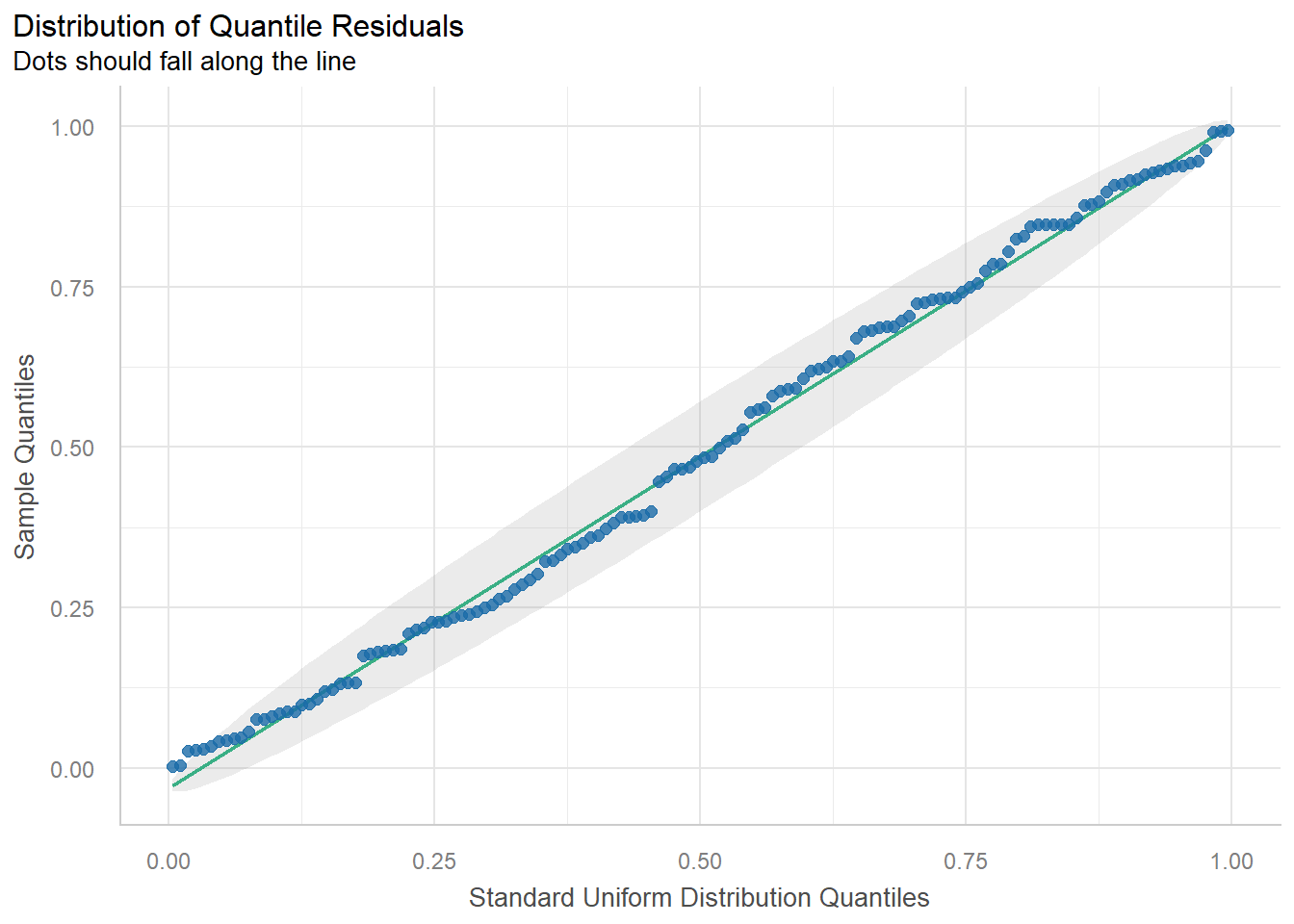
check_residuals(simulated_residuals) # testing the distribution of the quantile residuals against the uniform distribution using a Kolmogorov-Smirnov testOK: Simulated residuals appear as uniformly distributed (p = 0.756).Business as usual. We’re go to go!
performance’s simulate_residuals() function is basically a wrapper around the simulateResiduals() function from the DHARMA package. Sometimes, it can be interesting to directly look at the output of this function as it can provide a little bit of extra information!
DHARMa::simulateResiduals(dahu.res, n = 5000, plot = T)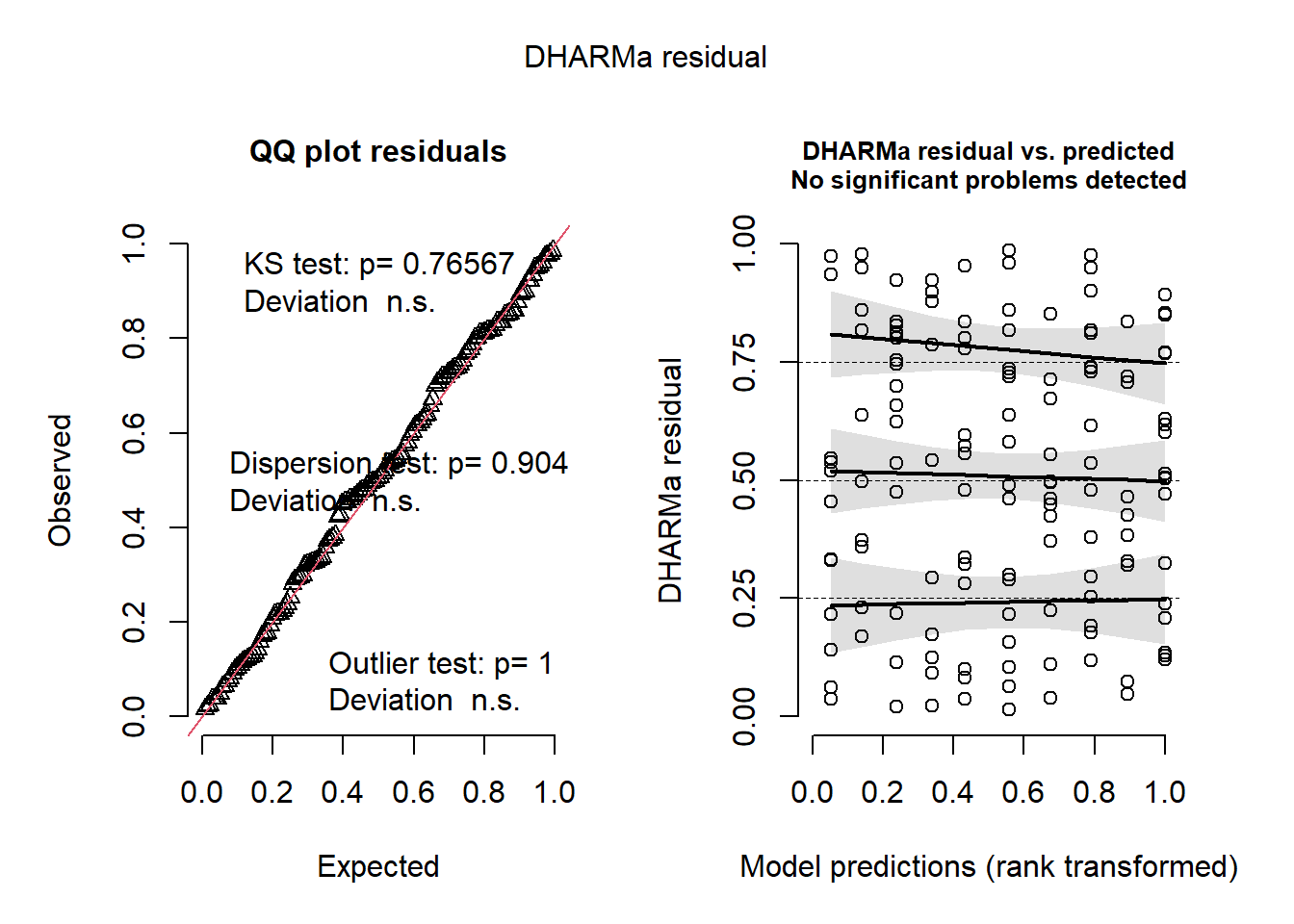
In the familiar linear regression, the coefficient of determination R2 is a common measure of goodness of fit. It represents the proportion of variance in the response variable explained by the predictors.Unfortunately, this cannot be used in the case of binary, nominal, or categorical response variables. But no matter, statisticians are not ones to give up on things that easily. While there is no uniquely agreed upon similar measure for logistic regression, several alternatives pseudo-R2 metrics have been offered.
One such example is McFadden’s R2 (but, again, there are several others). McFadden’s R2 ranges from 0 to just under 1. While values close to zero indicate that the model has poor to no predictive power, a McFadden’s R2 between 0.2 and 0.4 is often considered to indicate a very good model.
One way to compute this pseudo-R2 metric in R is through the aptly-named PseudoR2 function in the DescTools package. By default, when fed a model object, it only returns McFadden’s R2, but more can be obtained using the which argument.
library(DescTools)
PseudoR2(dahu.res,which="all")
McFadden McFaddenAdj CoxSnell Nagelkerke AldrichNelson
0.4136071 0.3929851 0.4361931 0.5817493 0.3642897
VeallZimmermann Efron McKelveyZavoina Tjur AIC
0.6272240 0.4793529 0.6567147 0.4800687 117.7408125
BIC logLik logLik0 G2
123.6240973 -56.8704062 -96.9834546 80.2260968 There are of course a lot more things that could be checked, inspected, looked at, refined, investigated, explored, and further scrutinized to your heart’s content, but for now, this should be enough to give you a good idea about whether or not your model is useful for inferences. Talking about inferences….
Let’s face it, we put up with the section above because we have to. This is a great opener, but this is not what we’re here for. What we want to do is listen to the soft whisper of our data revealing nature’s secrets to us. We want to be able to understand this marvelous world. We want to, dare I say, embrace our inner hubris and shade a light on the darkness of the unknown, navigate the uncharted, predict the future.
Let’s dive in the “piece de résistance”!
Summary — We have already seen how to extract some useful information from our model with the ever-so-useful summary() function:
summary(dahu.res)
Call:
glm(formula = detect ~ slope, family = binomial, data = dahu.data)

Coefficients:
            Estimate Std. Error z value Pr(>|z|)
(Intercept)  -1.0678     0.3069  -3.479 0.000503 ***
slope         2.0484     0.3362   6.093 1.11e-09 ***
---
Signif. codes:  0 '***' 0.001 '**' 0.01 '*' 0.05 '.' 0.1 ' ' 1

(Dispersion parameter for binomial family taken to be 1)

    Null deviance: 193.97  on 139  degrees of freedom
Residual deviance: 113.74  on 138  degrees of freedom
AIC: 117.74

Number of Fisher Scoring iterations: 5
Coefficients — R allows us to easily extract specific components of the output of the model with cookie-cutter functions. For example, we can extract coefficient values either directly from our model using coef():
coef(dahu.res)(Intercept) slope
-1.067753 2.048445 or from its summary (which provides a bit more details):
coef(summary(dahu.res)) Estimate Std. Error z value Pr(>|z|)
(Intercept) -1.067753 0.3069142 -3.478995 5.032984e-04
slope 2.048445 0.3361983 6.092968 1.108362e-09Confidence intervals — Confidence intervals can be calculated with confint():
confint(dahu.res) 2.5 % 97.5 %
(Intercept) -1.718622 -0.5044682
slope 1.446145 2.7691597p-values — And if p-values are your thing, they can also be extracted from the summary either directly, or from the reported coefficients as shown above:
summary(dahu.res)$coefficients[, 4] (Intercept) slope
5.032984e-04 1.108362e-09 coef(summary(dahu.res))[, "Pr(>|z|)"] (Intercept) slope
5.032984e-04 1.108362e-09 Personally, I am a visual guy, which is why I always appreciate a nice graph showing how our model fits the data. The general process to do so goes as follows:
First, get the results of the model (already done) .
Second, create a data frame containing the values of the explanatory variables for which we are trying to predict the response variable.
slope.new <- seq(min(dahu.data$slope), max(dahu.data$slope), length.out = 100)
expl.pred=data.frame(slope=slope.new) predict()” function with the model results and predictive variables. In the case of GLMs, the predicted response values are returned by default on the scale of the linear predictors (i.e. here the probabilities on logit scale, the log-odds). If we want to plot them, we will need to indicate to the function that we want to have our predictions on the same scale as the response variable (i.e. the ratio of “success” over the total number of trials). This is achieved by setting the argument “type” to the value “response”. The predict function now returns the success response probability in function of the explanatory variable.resp.pred <- predict(dahu.res, newdata=expl.pred, type="response")Now, we just have to plot all of that. Remember that the predict function returns fitted results on the probability scale, and therefore we are plotting the ratio of detection over the total number of sampling occasion (instead of simply the number of detections) in function of the covariate.
plot(prop~slope, data=dahu.prop,
     xlab = "Slope", ylab = "Detection rate")
lines(resp.pred ~ expl.pred$slope,col="red") # Fitted values
title(main="Dahu detection rate \nwith fitted logistic regression line")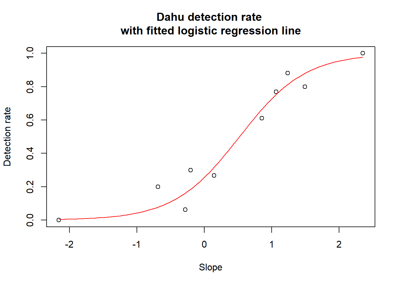
We can easily compute and add the prediction’s 95% confidence interval. To do so, first we compute the predicted values on the linear scale, and ask for the corresponding standard errors.
pred.linkscale <- predict(dahu.res, newdata=expl.pred, se=T)From there, we can approximate the 95% confidence interval on the linear scale, following the formula “95%CI= mean +/- 1.96*SE” (formula based on the normal distribution, assuming that the residuals are normally distributed on the linear scale).
pred.linkscale.CI2.5 = pred.linkscale$fit-1.96*pred.linkscale$se.fit # Lower CI 95%

pred.linkscale.CI97.5 = pred.linkscale$fit+1.96*pred.linkscale$se.fit # Upper CI 95%
Let’s back-transform from the linear scale to the response scale. To do that, we can feed the predicted values on the linear scale to the inverse link function. It’s possible to access the family used in the analysis with the function “family()”. This function takes as argument the object containing the GLM results, and returns (among other things) the inverse link function in the element “linkinv”.
pred.respScale.CI=data.frame(
   CI2.5= family(dahu.res)$linkinv(pred.linkscale.CI2.5),
   CI97.5= family(dahu.res)$linkinv(pred.linkscale.CI97.5)
   )
What’s left to do? Simply plot the corresponding lines!
plot(prop~slope, data=dahu.prop,
     xlab = "Slope", ylab = "Detection rate")
lines(resp.pred ~ expl.pred$slope,col="red") # Fitted values
title(main="Dahu detection rate with\nfitted logistic regression line")
lines(pred.respScale.CI$CI2.5 ~ expl.pred$slope,lty="dashed") # Lower CI 95%
lines(pred.respScale.CI$CI97.5 ~ expl.pred$slope,lty="dashed") # Upper CI 95%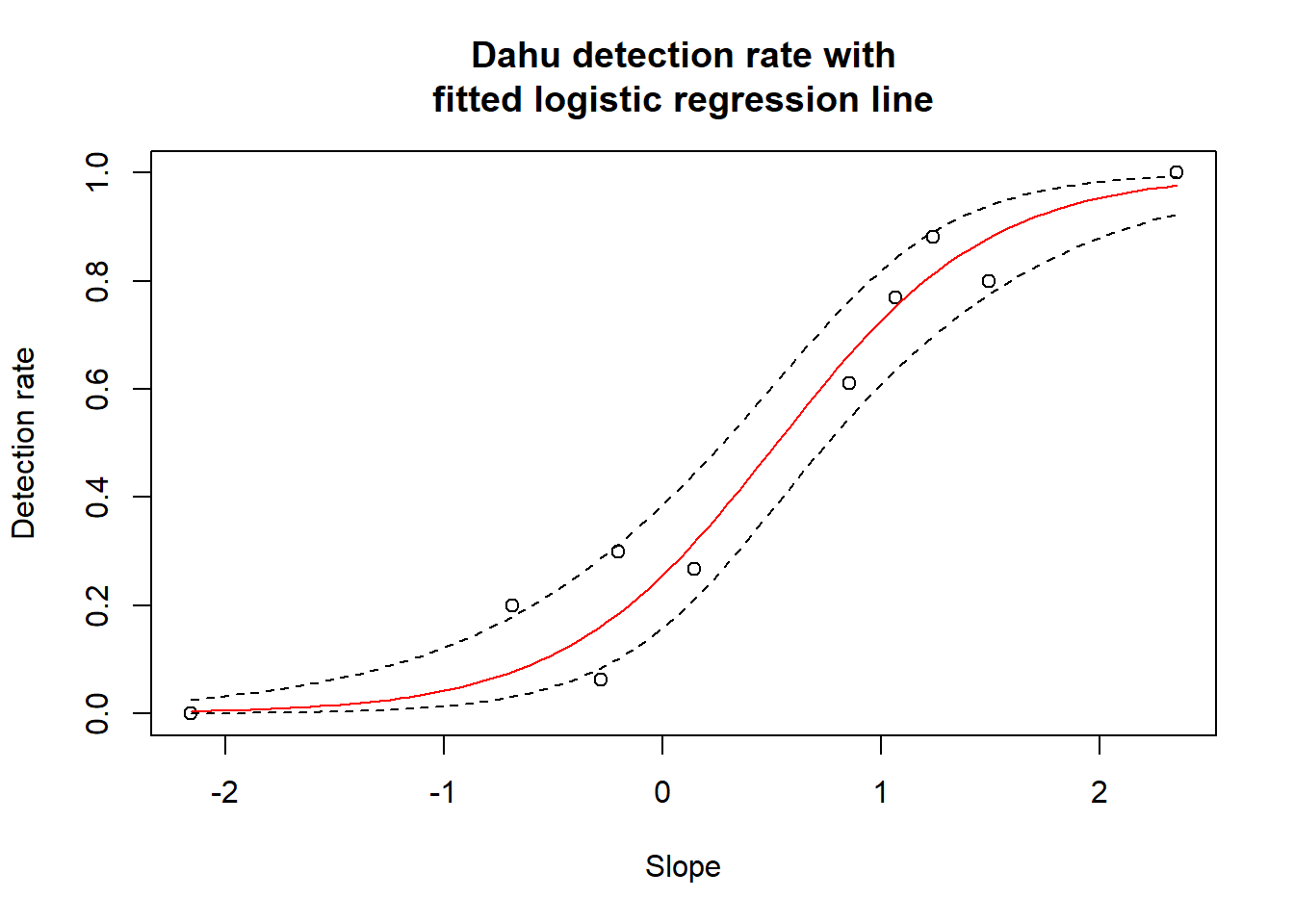
Not too shabby, is it?
Interpreting coefficients from the output of logistic regression is unfortunately not as straightforward as with a linear regression. Because we are using a logit link function to “linearize” the relationship between our covariates and the response variable, changes on the linear scale cannot readily be interpreted as changes of the response variable.
Let’s peak under the hood of our analysis. Remember the logit function?
\[\log(\frac{p}{(1-p)})\]
The logistic regression models the log-odds of an event. \({p}\) is our event probability, so \({1-p}\) is our probability of the event not happening. The ratio of the two is called the odds: how much more likely is the event to occur than not. Consequently, when we want to compare how the odds change in response to changes in our explanatory variables (e.g., scenario A vs scenario B), we can compare the ratio of the odds of our two scenarios. This is the odds-ratio!
In practice, this is obtained really easily by backtransforming our coefficients!
odds_ratios <- exp(coef(dahu.res))
odds_ratios
(Intercept) slope
0.3437802 7.7558350 Similarly, we can even get the confidence interval for the odds-ratio by calculating the confidence interval for our coefficients, and exponentiating it:
# Getting the coefficient confidence interval
ci <- confint(dahu.res)

odds_ratios_ci <- exp(cbind(OR = coef(dahu.res), ci))
odds_ratios_ci
OR 2.5 % 97.5 %
(Intercept) 0.3437802 0.179313 0.6038266
slope 7.7558350 4.246713 15.9452296Interpreting odds-ratio: Put simply, the odds-ratio (OR) represents the multiplicative change in the odds of the outcome occurring for a one-unit increase in the predictor variable, while holding all other variables constant.
Put simpler:
if OR = 1, there is no association between predictor and outcome,
if OR > 1, there is a positive association. Higher predictor values increase the odds of occurrence.
if OR < 1, : there is a negative association. Higher predictor values decrease the odds of occurrence.
In our case, for every one-unit increase in our slope covariate, the odds ratio of detecting a dahu increases by a factor of 7.76 [4.25 ; 15.95].
Another way of expressing the same information is to present the percentage change in odds-ratio, calculated as \(\Delta OR = (OR-1)*100\). Here, every one-unit increase in our slope covariate results in a 676% [325 ; 1495] increase in odds.
Finally, you can also streamline the odds-ratio computation using packages such as DescTools or oddsratio (I love it when developers use clear names for their packages).
Using DescTools:
DescTools::OddsRatio(dahu.res) # Notice the slight difference in CIs due to calculation methods
Call:
glm(formula = detect ~ slope, family = binomial, data = dahu.data)

Odds Ratios:
               or or.lci or.uci Pr(>|z|)
(Intercept) 0.344  0.188  0.627 5.03e-04 ***
slope       7.756  4.013 14.990 1.11e-09 ***
---
Signif. codes:  0 '***' 0.001 '**' 0.01 '*' 0.05 '.' 0.1 ' ' 1

Brier Score: 0.13     Nagelkerke R2: 0.582
Using oddsratio:
oddsratio::or_glm(dahu.data,dahu.res,incr=list(slope=1)) predictor oddsratio ci_low (2.5) ci_high (97.5) increment
1 slope 7.756 4.247 15.945 1With this, you should be good to go to tackle most GLMs involving Yes/No, 1/0, Detected/Non-detected data. As long as you know how to count to 1, you’re golden. What’s that? You passed Kindergarten and have decided that you shall not be restrained by such drastic constrictions? There are often more than one of one thing out there in the real world? … That’s fair…
I wonder if there is anything we could do about something like! (What a cliffhanger, hey?)