library(emmeans)8 Estimated Marginal Means
Model interpretation can sometimes feel like an art more than a science. And not like easy classical art either. More like weird modern French avant-garde scene art. As with any art piece, context is one of the most important thing to consider in order to understand the meaning of a work. In stats and modeling, it means that we cannot take raw data or even direct coefficient output from models at their face value. We need to interpret them with regard to the global conditions from which they emerge.
Estimated marginal means (EMM) are an essential tool to form a better picture of what a model actually means.
8.1 Concept
Estimated marginal means are estimated mean outcome for a particular group within a statistical model. Simply put, they provide a response prediction for a given factor/group level while controlling for other variables in the model. It is what makes them so crucial: the mean is adjusted to account for the influence of the other variables present in the model.
This adjustment is the reason why estimated marginal means provides a more accurate -and nuanced- understanding of the group’s average outcome by controlling for potential confounding factors.
In simple cases, with just a single factor and balanced designs, EMMs will be equal to the descriptive means. However, this is not the case anymore pretty much as soon as we include other variables.
In practice, EMMS will predict the response variable for a group or factor level by fixing all the other variables to a meaningful value (typically their respective averages), making comparisons between levels of the variable of interest possible.
Let’s imagine we are interested in the size of white-tailed deer in Florida. We have sampled two groups: females vs males. For each individual, we recorded the size and age. For some reason, we have a fairly imbalanced sampling when it comes to age. Most of our males are actually quite young, while our females are mostly fully adults. If we were to compare the mean size of each sex group using descriptive means, we would probably determine that on average, females are larger than males. However, if we were to fit the model size ~ age + sex, and then use the output of the model to predict average male and female sizes, while setting age to one specific common value (e.g., mean population age), we likely would see what we expected: males being larger than females.
This is particularly important when there are confounding variables or interactions between covariates.
In summary, EMMs control for the influence of other variables in the model, providing a more accurate estimate of group differences.
8.2 The emmeans package
In R, the best package to compute EMMs is probably emmeans. It is efficient and versatile, accepting multiple model types, and allowing for a lot of fine-tuning.
To demonstrate how to calculate EMMs, and even more importantly, how to interpret them, we are going to look at skunk ape abundance in 3 habitat types in Florida: forests, wetlands, and swamps. At each sampling location, we also recorded humidity levels.
skunk_ape.data <- read.csv("data/skunk_ape.csv")Let’s see what the raw descriptive means tell us…
library(ggplot2)

ggplot(skunk_ape.data, aes(x = hab, y = y)) +
  geom_bar(stat = "summary", fun = "mean") +
  stat_summary(fun.data = "mean_se", geom = "errorbar", width = 0.2)  +
  labs(x="Habitat",y="Counts",
       title="Skunk ape abundance in function of habitat type",
       subtitle ="Florida, USA") +
  theme_minimal() -> gg.skunk_ape

gg.skunk_ape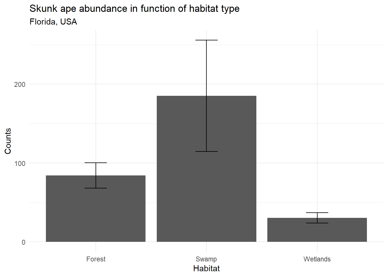
Ok, at first glance, it appears that skunk apes prefer swamps, feel “meh” about forests, and really don’t like wetlands.
The first step to verify this is to fit a GLM, modeling our response variable (counts) in function of the humidity levels and the habitat type:
skunk_ape.mod=glm(y~humidity+hab,"poisson",skunk_ape.data)

summary(skunk_ape.mod)
Call:
glm(formula = y ~ humidity + hab, family = "poisson", data = skunk_ape.data)

Coefficients:
            Estimate Std. Error z value Pr(>|z|)
(Intercept)  0.23829    0.05350   4.454 8.43e-06 ***
humidity     1.19501    0.01278  93.528  < 2e-16 ***
habSwamp     1.27378    0.02580  49.374  < 2e-16 ***
habWetlands  0.51144    0.03525  14.510  < 2e-16 ***
---
Signif. codes:  0 '***' 0.001 '**' 0.01 '*' 0.05 '.' 0.1 ' ' 1

(Dispersion parameter for poisson family taken to be 1)

    Null deviance: 14843.047  on 99  degrees of freedom
Residual deviance:    86.303  on 96  degrees of freedom
AIC: 614.11

Number of Fisher Scoring iterations: 4
A quick interpretation of our model output:
Our intercept is the forest habitat.
We detect a positive effect of humidity on counts.
Based on habitat coefficients, we can assume that skunk ape abundance is lower in the forests, highest in the swamps, and intermediate in wetlands.
EMMs are computed using emmeans(). The emmeans() function requires as input the fitted model, and a couple of settings. We need to specify the variable(s) for which we want to compare the predicted value, everything else will be kept constant. We can also specify on what scale we want our response variable to be: linear predictor scale (type = "link"), or back-transformed on the count scale (type = "response"). Most of the time, we will be more interested in the back-transformed values.
(emmeans_hab <- emmeans(skunk_ape.mod, ~ hab, type = "response")) hab rate SE df asymp.LCL asymp.UCL
Forest 17.6 0.516 Inf 16.6 18.6
Swamp 62.9 1.670 Inf 59.7 66.3
Wetlands 29.4 0.784 Inf 27.9 30.9
Confidence level used: 0.95
Intervals are back-transformed from the log scale Our EMMs indeed confirm our direct interpretation of the model output. Let’s see why it was so important to look at it from the marginal means point of view (i.e., estimates based on the statistical model) rather than from the descriptive means (i.e., solely based on the observed data). Here what the descriptive count means would have told us:
with(skunk_ape.data, tapply(y, hab, mean)) Forest Swamp Wetlands
84.40 185.15 30.58 What about a plot? Visual guy, remember?
# Descriptive means
gg.skunk_ape

# EMMs
plot(emmeans_hab, type="response",
     xlab= "Habitat", ylab = "EMMs",
     horizontal=F)
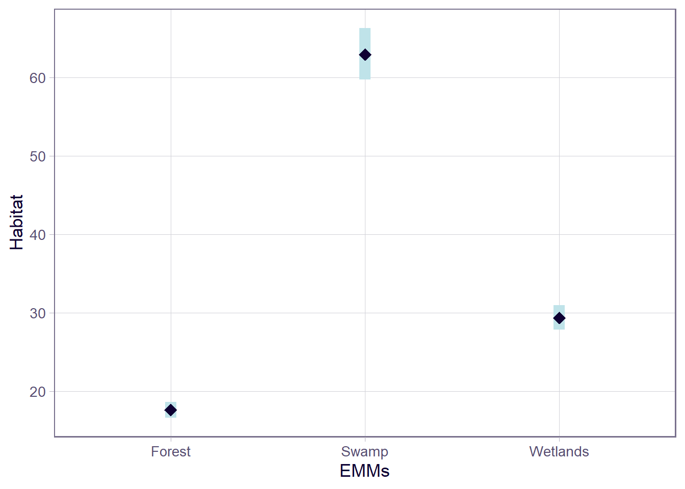
From those results, we would have incorrectly identified wetlands as the least welcoming habitat from skunk apes! Any guess why?… Remember, the EMMs fixed the other variables (here, humidity) to a common level between habitat types. Let’s see what the humidity levels in our observed data are for each habitat:
with(skunk_ape.data, tapply(humidity, hab, mean)) Forest Swamp Wetlands
3.040225 2.358412 1.634206 Oh. Wow. We have very different local humidity conditions. This is where our confounding effect came from: the effect of humidity hid the actual effect of habitat types! Good thing we caught that!
8.2.1 Plotting
We can directly plot our EMMs by converting the emmeans() output to a data frame:
library(ggplot2)

# Plot for River
emmeans_hab_df <- as.data.frame(emmeans_hab)

ggplot(emmeans_hab_df , aes(x = hab, y = rate, ymin = asymp.LCL, ymax = asymp.UCL)) +
  geom_pointrange() +
  labs(title = "Estimated Marginal Mean Counts by Habitat", y = "Count") +
  theme_minimal()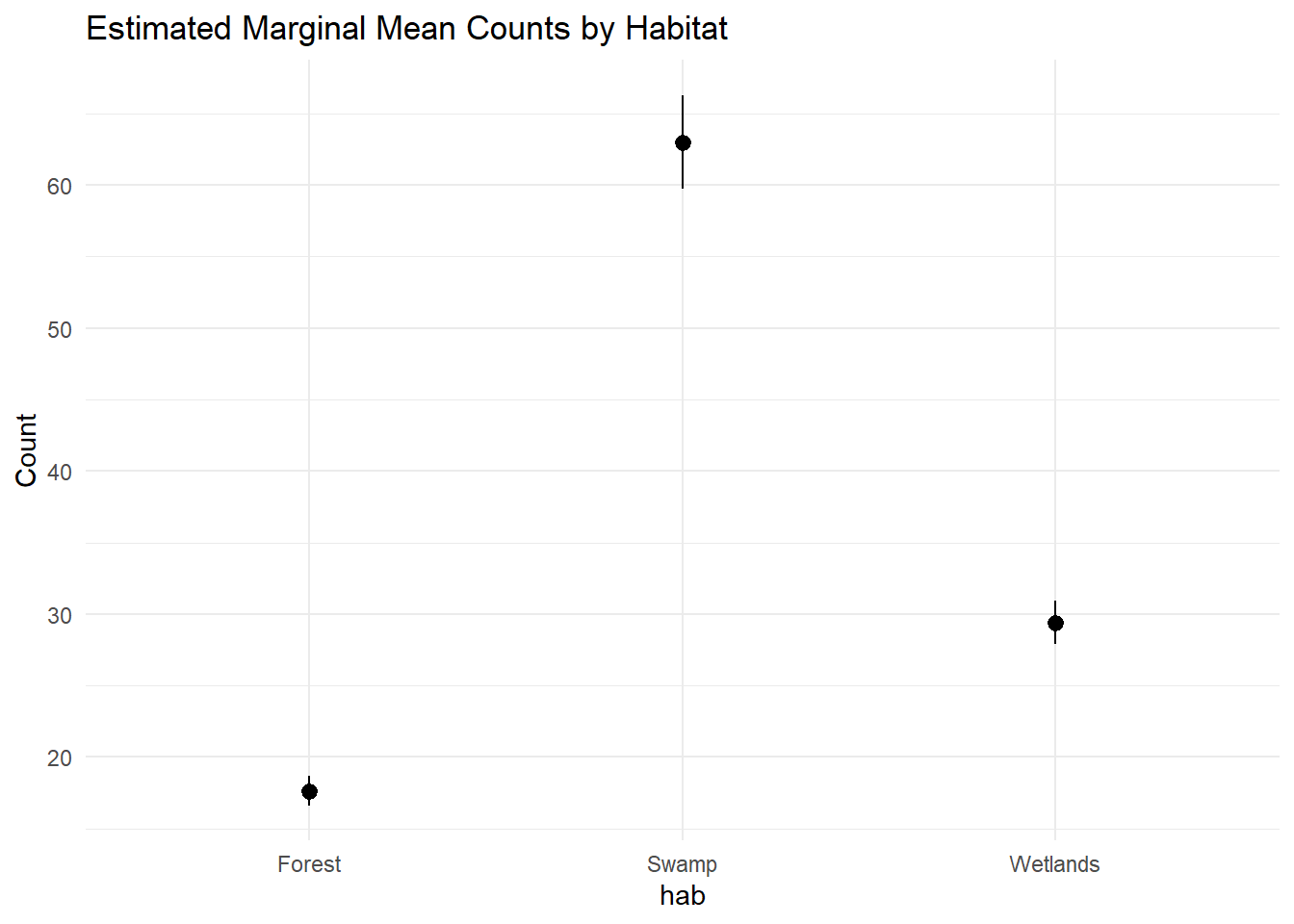
Or, by using the dedicated plotting function emmip from the emmeans package:
emmip(skunk_ape.mod, ~ hab | humidity, type="response" , CIs=T)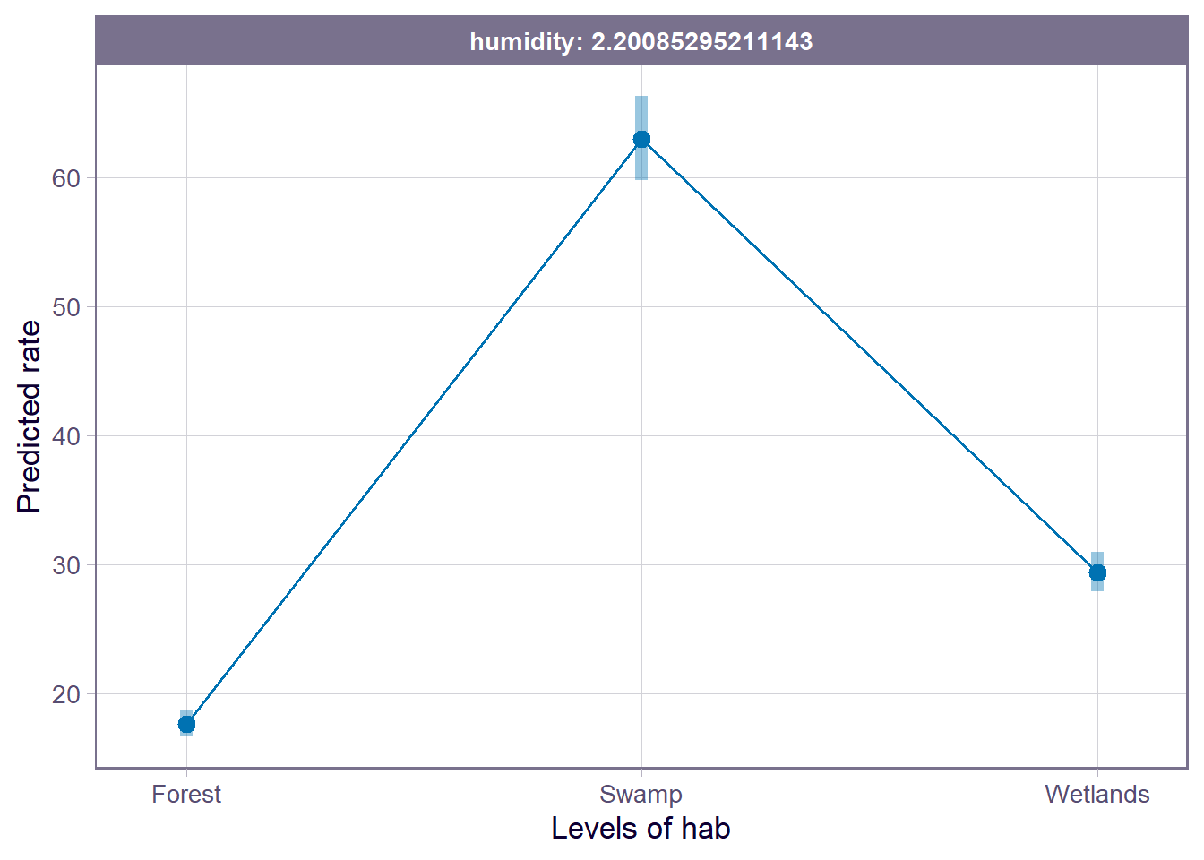
We can even include some information on the level at which humidity was set in order to compare habitat types (here, 2.200853)
8.2.2 Pairwise comparison
Finally, we can even compare our group levels in pairs to determine which level is preferred or more important, all the while testing to see if the differences are significant or not:
pairs(emmeans_hab) contrast ratio SE df null z.ratio p.value
Forest / Swamp 0.28 0.00722 Inf 1 -49.374 <0.0001
Forest / Wetlands 0.60 0.02110 Inf 1 -14.510 <0.0001
Swamp / Wetlands 2.14 0.07100 Inf 1 23.015 <0.0001
P value adjustment: tukey method for comparing a family of 3 estimates
Tests are performed on the log scale Note that pairs() automatically adjusts p-values to account for the repeated tests!